Non Covalent Interactions from Promolecular Densities

This tutorial shows how the promolecule module in QC-AtomDB can be used to calculate the reduced density gradient of a molecule.

Non covalent interactions (NCI) such as hydrogen bonds, van der Waals interactions and steric clashes, play a central role in the structure and properties of (macro)molecules. The reduced density gradient, \(s(\mathbf{r})\), is an aproach to identify such interactions as distinguishable features in real space. \(s(\mathbf{r})\) is defined as a ratio of the gradient of the electron density to the electron density itself:

\[s(\mathbf{r}) = \frac{1}{2(3\pi^2)^{1/3}}\frac{|\nabla \rho (\mathbf{r})|}{\rho^{4/3}(\mathbf{r})}\]

For big molecular systems (such as biomolecules or materials), the calculation of the reduced density gradient is computationally expensive. The promolecule module in QC-AtomDB is a fast alternative to get the necessary ingredients to calculate the reduced density gradient in terms of promolecular density properties. These are properties of a molecule evaluated from the linear combination of the properties of the atoms that compose it. For example, the promolecular density is defined as:

\[\rho^{mol}_{pro} = \sum^{N_{atoms}}_{i=1} c_i \rho^{atom}_i\]

These atomic densities are obtained from the atomic densities database in QC-AtomDB.

As model systems the water molecule and its dimer will be used:

drawing

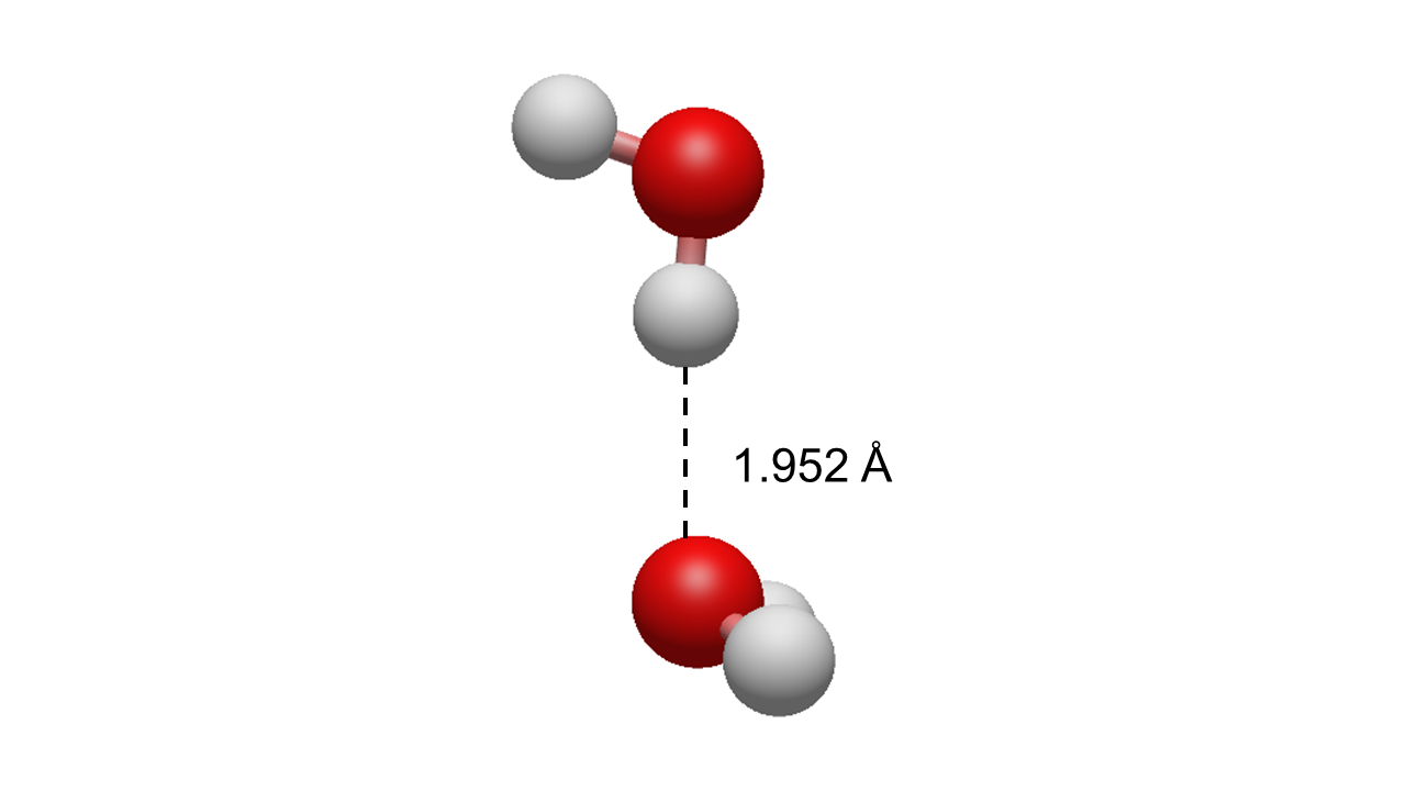
By plotting \(s(\mathbf{r})\) versus \(\rho(\mathbf{r})\), and analysing the low density region, the presence of non-covalent interactions in the dimer can be identified. To further clasify the type of the interaction one needs to look at the sign of the laplacian of the density, which we do not cover here.

Then, to compute the reduced density gradient one needs: - Molecular coordinate file (e.g. XYZ file) - Cubic grid of points - Electron density and density gradient at points

As a way to also demonstrate the seamles interface between AtomDB and other packages in the QC-Devs environment, we will use modules from IOData and Grid to read the molecular coordinate files and generate the grid of points, respectively.

Packages install for Google Colab

[ ]:

# ! pip install git+https://github.com/theochem/iodata.git
# ! pip install git+https://github.com/theochem/grid.git
# ! pip install git+https://github.com/theochem/AtomDB.git@tutor_notebooks

[ ]:

# # download the example files
# import os
# from urllib.request import urlretrieve

# fpath = "data/"
# if not os.path.exists(fpath):
#     os.makedirs(fpath, exist_ok=True)

# urlretrieve(
#     "https://raw.githubusercontent.com/theochem/AtomDB/dev/examples/notebooks/data/h2o_dimer.xyz",
#     os.path.join(fpath, "h2o_dimer.xyz")
#     )

# urlretrieve(
#     "https://raw.githubusercontent.com/theochem/AtomDB/dev/examples/notebooks/data/h2o_promol_rho.npy",
#     os.path.join(fpath, "h2o_promol_rho.npy")
#     )

# urlretrieve(
#     "https://raw.githubusercontent.com/theochem/AtomDB/dev/examples/notebooks/data/h2o_promol_reducedgradient.npy",
#     os.path.join(fpath, "h2o_promol_reducedgradient.npy")
#     )

[ ]:

# Optional modules
import numpy as np
import matplotlib.pyplot as plt
from iodata import load_one
from grid.cubic import UniformGrid
# AtomDB's promolecule tool
from atomdb import make_promolecule


# Function to evaluate the reduced density gradient
def reduced_density_gradient(rho, nablarho):
    coeff = 2 * (3 * np.pi ** 2) ** (1 / 3)
    gradnorm = np.linalg.norm(nablarho, axis=1)
    return gradnorm / (coeff * rho ** (4 / 3))

# Load the coordinates of the water dimer
fname = 'h2o'
mol = load_one(f'data/{fname}_dimer.xyz')
atnums = mol.atnums
atcoords = mol.atcoords # in Bohr

# Generate a 3D grid with a spacing of 0.2 Bohr and an extension of 5.0 Bohr
cubgrid = UniformGrid.from_molecule(atnums, atcoords, spacing=0.2, extension=5.0, rotate=False, weight="Trapezoid")

# Build de promolecule and evaluate its density and gradient. The 'slater' dataset is used to obtain the atomic data
dimer_promol = make_promolecule(atnums, atcoords, dataset='slater')
dimer_rho = dimer_promol.density(cubgrid.points, log=True)
dimer_grad = dimer_promol.gradient(cubgrid.points, log=True)

# Compute reduced gradient
dimer_rdgrad = reduced_density_gradient(dimer_rho, dimer_grad)

# Load density and reduced density data for a single H2O molecule
h2o_rho = np.load(f'data/{fname}_promol_rho.npy')
h2o_rdgrad = np.load(f'data/{fname}_promol_reducedgradient.npy')

# Plot the reduced gradient as a function of the density
plt.scatter(dimer_rho, dimer_rdgrad, label='H2O dimer')
plt.scatter(h2o_rho, h2o_rdgrad, label='H2O')
plt.xlim(0., 0.3)
plt.ylim(0., 1.0)
plt.xlabel(r'$\rho(R)$')
plt.ylabel(r'Reduced gradient')
plt.legend()
plt.show()