Promolecule properties

AtomDB provides basic functionality to compute promolecular properties from the atomic data. The tool is called promolecule. The module offers evaluation of intensive and extensive properties with the tool function make_promolecule.

Building a promolecule

Creating a promolecule is as simple as providing the list of elements and coordinates defining the molecule as is shown here for the Berillium dimer. Additionally, the source of atomic properties is required, which in this case is the slater database.

[1]:

import numpy as np
from atomdb import make_promolecule


# Atomic numbers of each center
atnums = [4, 4]

# Spatial coordinates of each center
atcoords = np.asarray([
    [0., 0., 0.],
    [0., 0., 2.],
], dtype=float)


# Make promolecule instance
promol = make_promolecule(atnums, atcoords, dataset='slater')

Extensive (global) properties

\[P^{mol}_{pro} = \sum^{N_{atoms}}_{i=1} c_i P^{atom}_i\]

where \(P^{atom}_i\) are the atomic properties and \(c_i\) are the coefficients.

[2]:

print("\nProperties:")
# print(f"Nelec  \t{promol.nelec():+.6f}")
# print(f"Nspin  \t{promol.nspin():+.6f}")
print(f"Mass   \t{promol.mass():.6f}")
print(f"Energy \t{promol.energy():.6f}")


Properties:
Mass    18.024366
Energy  29.146046

Extensive (local) properties: density properties

[6]:

# Construct a 3D grid along the z-axis of the linear molecule
N = 2000
rad_grid = np.linspace(-3., 5., num=N)
grid = np.zeros((N, 3))
grid[:,2] = rad_grid

# Compute the density and kinetic energy density at the points
promol_dens = promol.density(grid, spin='ab', log=True)
promol_ked = promol.ked(grid, spin='ab', log=False)
promol_grad = promol.gradient(grid, spin='ab', log=False)
promol_lapl = promol.laplacian(grid, spin='ab', log=False)
promol_hess = promol.hessian(grid, spin='ab', log=False)

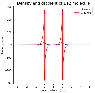
Visualizing density properties

[17]:

import matplotlib.pyplot as plt

fig = plt.figure(figsize=(6, 6))
ax = fig.add_subplot()

ax.plot(rad_grid, promol_dens, color="blue", label="Density")
ax.plot(rad_grid, promol_grad[:,2], color="red", label="Gradient")
ax.set_xlabel("Radial distance (a.u.)")
ax.set_ylabel("Property value")
ax.legend()
ax.set_title("Density and gradient of Be2 molecule", fontsize=16)
plt.show()

../_images/notebooks_Promolecule_Tools_8_0.png

Intensive properties

\[\langle P \rangle_p = \left(\frac{1}{n}\sum_{k=1}^n P_k^p \right)^{\tfrac{1}{p}}\]

where \(P_k^p\) are the atomic properties and \(p\) is the power of the average.

[19]:

# print("\nProperties:")
# print(f"Promolecule IP (eV) \t{promol.ip(p=1):.6f}", ) # not supported by Slater dataset

Promolecule with floating point charges and/or multiplicities

When defining a promolecule, the charges and multiplicities of the atomic species can be specified as through the charges and mults arguments. These can be either integers or floats. When the values of these variables are floats, …

Note that if one of (charges|mults) is a float and the other is an integer, we also interpolate.

[ ]:

# Charges of each center
# (integer to directly use a species, float to interpolate)
charges = [1.2, 0]

# Multiplicities of each center
# (integer to directly use a species, float to interpolate)
# (positive for spin-up, negative for spin-down)
mults = [-1.2, 1]

# Build a promolecule
promol = make_promolecule(
    atnums,
    atcoords,
    charges=charges,
    mults=mults,
    units="bohr",
    dataset="uhf_augccpvdz",
)

print("\nProperties:")
# print(f"Nelec  \t{promol.nelec():+.6f}")
# print(f"Nspin  \t{promol.nspin():+.6f}")
print(f"Mass   \t{promol.mass():.6f}")
print(f"Energy \t{promol.energy():.6f}")